Linux kernel as described in my previous writing has 3 major watermarks, High, Min and Low. This blog is a brief view of the watermark calculation in the Linux system.
1. Use variable from admin window /proc/sys/vm/min_free_kbytes
Converts kbytes unit to page unit.
pages_min = min_free_kbytes >> (PAGE_SHIFT – 10);
2. Calculate total managed pages in each zone except highmem zone( if it exists )
For Each zone calculate the following 3. Calculate fraction for each zone’s pages_min with respect to lowmem_pages. tmp= ( pages_min / lowmem_pages ) * zone->managed_pages.
Managed_pages are total available page count in a zone that could be used for allocation.
4. Calculate WMARK_MIN for HIGHMEM using following calculation:
min_pages = zone->managed_pages / 1024
min_pages = MIN( MAX(min_pages, SWAP_CLUSTER_MAX), 128)
5. Else, simply use the tmp variable as min_pages watermark count.
6. Calculate the distance for the rest of the watermarks.
Its the fraction of managed_pages by 10000, scaled by watermark_scale_factor = 10
fraction = ( zone->managed_pages / 10000 ) * watermark_scale_factor
distance = MAX( tmp >> 2, fraction);
This series of articles tries a hand on hand analysis of memory management policies accommodated in acclaimed Unix-like operating systems like OpenSolaris, FreeBSD with Linux.
Memory management conventionally has three major policies.
Fetch Policy: When to fetch a page from auxiliary memory.
Placement Policy: Where to place the fetched page in main memory.
Replacement Policy: Which page to replace in case of memory shortage.
The mentioned policies are well studied and reasoned( Though I will write on this as well), nevertheless another policy which directly impacts the performance of a system is scan rate policy.
Rest of this specific work will focus on this policy and its approach in different operating system.
What is a scan rate policy?
Operating systems keeps updating the position of the allocated pages in their corresponding list based on its access frequency and other parameters. This enables the replacement policy to fetch the pages based on the position for replacement. Scanning through the entire list of allocated pages and updating the position of every page each time is an expensive operation. To avoid such a colossal expense, operating systems will only scan a portion of the list at a given moment of time and updates the corresponding page’s position. The policy that decides on the fraction to scan at a given instance of time is termed as scan rate policy.
Generalities in the model. Habitually on nearing a particular distance to exhaustion, the system starts a kernel level daemon, that runs in concurrence with other processes, termed either as pageout daemon( OpenSolaris and OpenBSD) or Kswapd daemon( Linux); Albeit the name of the process changes based on platform implementation, its intention remains the same .i.e., scan a certain amount of pages, apply the desired replacement policy and evict a set of pages to leeway for the current memory need. The free list of pages might have many waypoints in between the list called watermark. In Common, watermark decides on when to start the scan, rate of scan, number of times to scan, amount of processor utilisation page scanner can take( called CPU CAP), amount of I/O utilisation page scanner can use( called I/O CAP), etc., but the mentioned set varies both in implementation and inclusion based on the platform of implementation. Extensively, many operating systems quantify the measure of watermarks in page numbers.
Implementation In OpenSolaris:
OpenSolaris uses watermark based policy, i.e., scan rate policy changes based on the watermark .
Model. OpenSolaris have three major watermarks, namely lotsfree, desmem, minfree. The system has two different scan policies called slow scan and fast scan. The system also have two different rate at which the scanning will happen per second, i.e., 4times/second and 100times/second. Further, Solaris restricts the CPU utilisation of the page scanner between 4( min_percent_cpu) to 80( max_percent_cpu) percent( Used as a scaling factor) and the I/O is capped at either 40 or 60 IO/second( maxpgio ), but this restriction is based on the formulae , Intuitively it means busy on disk arm is all that is tolerable for paging.
By default lotsfree is of total memory, desmem is of lotsfree and minfree is of desmem. Fast scan is scaled to and slow scan is hardcoded with 100. The whole of this value initialisation is done in function setupclock.
Another watermark worth mentioning is throttlefree. This watermark in general is equated with minfree.
Fig1: OpenSolaris Scan Rate With Respect to Watermark
Policy. Once memory reaches lotsfree watermark, pageout daemon kickstarts. The amount of page to scan is determined by the formulae:
where freeMem mentions the current instance of free memory in quantity of pages. Intuitively intial values of scan rate is majorly contributed by slow scan, but as it nears the exhaustion fastscan’s value starts increasing and contributing towards scanrate.
CPU utilisation is interpolated with the scanrate by sporadic check and comparison of the time taken to scan n pages ( called PAGES_POLL_MASK hard coded with 1023)with the utilisation.
Basically the fraction of memory available with respect to lotsfree is scaled to the ScalingFactor of CPU.
Between lotsfree and desfree the memory is scanned 4 times/second. Once the memory reaches less than desfree its scanned 100 times/second.
The throttleFree watermark suspends the allocation of pages that has the wait flag set till scanner brings the memory back above minsfree.
P.S. The same logic is implemented in 4.3BSD, but lotsfree is of total memory, desfree is of lotsfree and minfree is of desfree.
Implementation in FreeBSD:
FreeBSD have a much simple scan policy compared to Solaris and 4.3BSD. The watermarks are replaced by a minimum percent of memory that needs to be maintained. If the memory reaches below this threshold then pageout daemon is started.
Model. FreeBSD divides the pages into 5 categories of pools, namely wired, active, inactive, cache and free. Pages that are unmovable from the physical memory are named wired, pages that is currently part of active execution is called active, pages that are not part of active execution is called inactive, pages that are not used anymore are cached and pages that are not allocated is in free list.
Policy. The system has 2 thresholds, namely minimum and target thresholds. The systems goal is to maintain a minimum threshold of pages in active, cache and freelist, Once the pages reach below the minimum threshold then the pageout daemon kickstarts and starts pushing the pages back to target threshold. By default the values are:
Free + Cache( free_target) : 3.7% and 9%
inactive( Inactive_target): 0% and 4.5%
But these values are modifiable through user level interfaces.
Procedure:
Pageout daemon calculates the minimum required pages that are needed to get above the threshold.
Tries to acquire the required pages through 3 passes.
page_shortage = free_target – (free_count + cache_count). Tries to acquire this target. If the achieved target does not satisfy the needed target, then we move to pass 2.
page_shortage = ( free_target + inactive_target) – ( free_count + cache_count + inactive_count). Tries to acquire this target. If the achieved target does not satisfy the needed, then we move to pass 3.
kickstart swap out daemon, still all memory is full, then kill the biggest memory consumed process.
After the 1st pass check the time difference between previous pass and current pass. If the difference is more than lowmem_period(10), then trigger vm_lowmem event. This event tries to decrease many other registered cache sizes and reclaims the same.
Implementation in Linux:
Linux uses watermark amalgamated with demand based scanning, i.e., on allocating a page, the watermark is tested and if the current watermark before the allocation is less than the desired, then try reclaiming the zone directly and also start kswapd if required. The scan amount is based on user defined parameter called swappiness . The reclamation policy is
Model. The Memory( A node in NUMA based machines) is basically divided into zones. Each zone has High, Low and Min watermark. The ratio of the watermarks can be set by the user. Scan rate is determined by variable called swappiness, default value is 60, but can also be set by user, maximum value recommended is 100.
Fig2: Linux Scan Rate With Respect To Watermarks
Policy.
Before allocation, test for Min watermark is made by adding the allocation order count of the request to free page count. If pages are below the low watermark and GFP is not either set to GFP_MEMALLOC, then direct reclamation of the zone is tried with the count of SWAP_CLUSTER_MAX, provided GFP_DIRECT_RECLAIM is set for the allocation request.
If the GFP is set with GFP_KSWAPD_RECLAIM, then kswapd is triggered to reclaim MAX( SWAP_CLUSTER_MAX, high watermark).
If the watermark falls below Min watermark then synchronous direct reclamation is attempted, i.e., any allocation request for pages with GFP_WAIT set is suspended on the wait queue. Concurrently kswapd tries to bring back the pages above high watermark.
In both the cases reclaim uses the following mechanism to scan the pages.
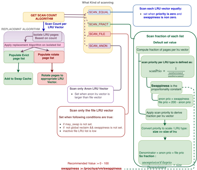
The variable named priorityscan_controldecides on the portion of the zone to scan.
Pressure is applied on each zone on file or anon lru formulae derived as:
.
.
respective pressure is either anonyomous or file page priority.
Fraction per list Computation
Denominator = ap + fp .
Numerator = ap (or) fp.
Fraction to scan = .
Scaling: Fraction to scan is scaled to scan_portion
Scan_amount = Fraction to scan * Scan_portion.
Basically, scan portion is scaled to the fraction we derived.
If the priority is zero and swappiness are non-zero, then Scan count is set to SCAN_EQUAL. This means the ignore the fraction calculation and directly derive the scan count based on the priority for each inactive list.
P.S. The statistical variables rotated and scanned is decomposed to half once it reaches a threshold.
intuitively, it is a heuristical thought that reasons with a belief that more the pages are rotated( see Second Chance Algorithm) in a particular lru list then the possibility to reclaim pages from the same are less. Finally, it’s worth to note that described policies are simplified to provide clarity on the core idea.
Detail Description Of Linux Scan count determination.
This issue is continuation of previous instalment, i.e. on Simple List Of Blocks. In previous section we saw the logical perspective of SLOB, In this section we would look into the implementation perspective of SLOB.
Data Structure. To start with, lets first derive data structure necessary to make the implementation work.Usually, the correct selection of data structure is the key to designing a good algorithm. To design for SLOB we primarily need two data structures, one is the list holding the chunks of same size and other to hold the chunk frame itself.
The List. Each element in the list needs to be a collection holding at least two elements, namely a variable holding the size of the chunks and other holding the head of the chunk frames. The list we are intending to design could be of two kinds; contiguous and disjoint. Both has its own advantages and disadvantages; the list being contiguous saves space of holding reference to the next element, but at the same time prevents the list from further expansion. In this implementation we would design blocks as disjoint linked list and list as contiguous. This approach imitates the implementation of many real libraries.
struct list {
    unsigned int size; /// holds the size of the blocks.
    void *head;  /// head of list of blocks.
};
The Blocks. When noticed from implementation perspective, the blocks are simply a list that grows and shrinks in horizontal direction, whereas the list holding blocks is represented vertically remains constant. To understand the data structure that defines the notion of blocks , its basically a collection holding a header element, data and a reference to the next element in the list, else next holds NULL. Creating this structure is quite tricky, which we would discuss in the coming sections. For now we will just stick with the declaration of data structure.
struct block {
     struct list *lst; ///the reference to the list the block belongs.
     struct block *nxt; ///reference to nxt block in the list.
     void *block;  ///The block or payload itself.
};
The beginning of the structure holds the reference to the list to which the block belongs, this enables the return to the list( free) a constant operation, then the list holding the reference to the next block, finally the chunk itself which would be returned to the user on malloc.
Construction of Data structure. Before we start addressing the construction of data structure, we need to think of an approach of calling an init function before the main() function.Calling init before main() provides an abstract view of the library calls. Moreover this is the approach almost all library level implementation follows .
To make this work, GCC has a set of compiler directives named as attributes. The attributes extend the language syntax .i.e. Basically instructs the compiler of how the particular function or variable should be altered during compilation or linking phase. To define a attribute:
__attribute__((attribute_list)) <function or variable>.
Of many attribute_list our area of interest is constructor and destructor.
From horse mouth : “The constructor attribute causes the function to be called automatically before execution enters main (). Similarly, the destructor attribute causes the function to be called automatically after main () has completed or exit () has been called”.
To understand the working of the mentioned attributes, let me make a confession about main(). The main is not the first function to execute when you start executing a process, rather there are many other preparation functionalities that execute before and after main().
so giving a rough view of how the main looks in whole picture is
_start     // First symbol to start execution of a process
.        // stored at location 0x080482d0
.
.
call constructors
ret = main();
call destructors
.
.
copy the ret value into parent
signal parent with sigchld
Though real implementation is much more complex, I presume this level of explanation would suffice for getting a pictorial understanding.
To make this work, the shared object file contains special sections (.ctors and .dtors on ELF) which contain references to the functions marked with the constructor and destructor attributes, respectively. When the library is loaded/unloaded the dynamic loader program (ld.so ) checks whether such sections exist, and if so, calls the functions referenced therein.
Now lets get back to our implementation on construction of data structure. Rough sketch of the implementation would be
create a contiguous list, i.e. an array of list based on number of heterogeneous blocks needed by the process.
For creating each set of homogeneous block, call sbrk() with size as(sizeof(header)+ BLOCK_SIZE) * number of blocks in the set.
now dissect each allocated block into piece of chunk frames.
Lets make this into a small snippet, where initialisation is done with single element on the list.
#define SLOB_LEN 1
struct list slob[SLOB_LEN];

__attribute__((constructor)) void init(void)
{
    int i = 0;
    do {
        slob[i].size = 8; /// hard coded for simplicity
        slob[i].head = make_blocks(8, 2, &slob[i]);
        i++;
     } while(i < SLOB_LEN);
}

/*
  @ FUNCTION NAME: make_blocks
  @ DESCRIPTION: makes the blocks with given specifications
  @ INPUT: block_size: size of the block
           no_of_blks: count of the blocks
           list      : list to which the block belongs
  @ OUTPUT: returns the starting address of the blocks created
*/
void* make_blocks(const int block_size, const int no_of_blks, struct list* list)
{
    void *chnk = sbrk((block_size + sizeof(struct list)) * no_of_blks);
    int i = 0;
    struct block *blks = NULL;

    do {
        struct block *tmp = (struct block*) chnk;  //type cast chnk into header

        /* Header construction*/
        tmp->lst = list;
        tmp->nxt = blk;
        /* Block itself*/
        tmp->block = tmp + 1;
        /* prepend to the list*/
        blks = tmp;

        chnk = chnk + (sizeof(struct block) + block_size);
        i++;
    } while(i < no_of_blks);
    return blks;
}
This might look little complicated on first sight but on second glance I can guarantee that its pretty straight forward.
Malloc. This is pretty straightforward, just iterate through the list to find the size that best suits. The SLOB is also best fit, because the list would be arranged in ascending order.
void* Malloc(const int size)
{
   int i = 0;
   void *p = NULL;
   do{
      if(slob[i].size >= size) {
         if(slob[i].head) {
             p = slob[i].head->block;
             slob[i].head = slob[i].head->nxt;
         }
      }
i++;
   }while(i < SLOB_LEN);
   return p;
}
Free. The field in the struct block holding the reference to the list enables return to the list in constant time.
The previous section helped us understand two major syscalls namely brk and sbrk. I also implemented a basic malloc technique using these syscalls and addressed the problem on direct accessing these syscalls, i.e. The order of Free should be exact reverse of malloc, else would lead to segmentation violation.
Another problem worth mentioning is, system calls are expensive due to context switch between kernel space and user space; Moreover this might also lead to unnecessary suspension of process.
Approach to solution. To address the mentioned problems we should reduce the number of time syscall’s is made and secondly rather than reverting or contracting the data segment we should create a hole in the heap which could be reused.
Solution. To make the above challenges addressable we need to use a notion called memory pooling, i.e. pre-fetch a big chunk of memory and cut a piece from it when required. This cut piece is given back to the chunk on free function( not given back to the Kernel, but rather pooled).
Challenge. The mentioned solution is not straight forward; first allocation should not provide you with memory very big compared to the requested size( causing Internal Fragmentation) and the time taken to process the request should be reasonable. Second the freeing of memory should happen in constant time, i.e.O(1).
Simplest solution that addresses the mentioned challenges is SLOB, i.e. Simple List Of Blocks. As name suggests its a list holding reference to “set of chunks” of same size.The list is arranged in ascending order based on size of the chunk it holds.To make this approach work, the memory needed for the process is approximately precomputed , prefetched and made into SLOB before main function is called.
The Above figure is a simple representation of SLOB.
On Malloc the list is searched for the first fit( which in SLOB is also the best fit because of its ascending property). If the desired requested size can be allocated, then the chunk is removed from the list and its starting address is returned, else NULL is returned. The complexity of the fetch is O(N), where N is the length of the list, i.e. linear complexity.
Free just takes the starting address of the chunk and provides no other information about the size or other information about the cache( or element) to which the chunk belongs; but on free the released chunk needs to identify the desired cache to which the chunk belongs.With just starting address as parameter,it is not possible to return the chunk to the desired cache in constant time, unless the chunk holds some reference of the ownership. To make this work a notion called boundary tag is used.
Boundary tag: Either before or after each chunk a record is added, holding the reference of the element to which the chunk belongs. This boundary tag is provided to each chunk. The total size of each chunk is chunk-size + boundary tag. The size of the boundary tag is of great importance; Bigger it becomes , overhead of book keeping data becomes proportionately larger, but at the same time the size should be efficient enough to hold required data so that chunk can be returned to the respective element it belongs. Study suggests that boundary tag should not be greater than 10% of the total payload memory. To implement SLOB the size of the tag would be a word length, i.e. 32bits in case of 32bit system to hold the reference of the owned element.
The diagram on the left is an abridged representation of the boundary tag.
Abstraction.When malloced the address at the end of the tag is returned; therefore, the user is abstracted from underneath implementation of the allocation.
In many scientific publications the boundary tagging is called hidden header field.
when free is called it gets end address of the boundary tag, i.e. the starting address of the chunk. To this address when the size of the boundary tag is negated we would get the reference of the chunk’s tag. This provides us with the required information about the element to which the chunk should be returned. The complexity of the Free is O(1).
Usage:
This notion of SLOB is used in many RTOS that works on flat memory model. among many, One worth mentioning is OSE166’s redarrow platform. This platform was majorly used on many primitive mobile devices.
Another place with prominent usage is SLAB implementation in Linux kernel; Where the kernel data structures are alloced using such an implementation, but with a slight twist; which we will discuss in much detail as we progress.
Many Middlewares uses this approach to build a wrapper around the standard library to make access to memory faster.
Conclusion.This article provided us the semantic understanding of SLOB, In the next article we would discuss a method to implement the SLOB and would also discuss the pros and cons of this algorithm.
Definitions used in this articles:
Internal fragmentation: is the wasted space within each allocated block because of rounding up from the actual requested allocation to the allocation granularity.
Flat memory model or linear memory model refers to a memory addressing paradigm in which “memory appears to the program as a single contiguous address space.”The CPU can directly (and linearly) address all of the available memory locations without having to resort to any sort of memory segmentation or paging schemes.
The Word Dynamism in memory has always been a fascinating area to understand. For many beginner level programmers, the allocation of dynamic memory using library calls like malloc have been a magic like complex implementation.
This series of articles tries to provide a profound insight on how the dynamic allocation works. The article starts with very basic implementation and walks towards an advanced version which is currently used in large servers, embedded devices and general purpose operating systems.
The whole article uses Linux as the basis to explain the dynamic allocation.
To start with, let’s try to understand the need for such a dynamic mechanism; Assume user has to enter an input for a programme, which in turn is just a reference to a file holding variable length data, but the length is not known in advance. This scenario could be effectively handled with dynamic allocation, else programmer have to pre compute maximum needed data length and statically allocate them. This static allocation leads to unnecessary blow up of programme size. Other scenarios like reading data from sensors whose lifetime is short lived; but the length of the data produced is not known in advance would be justified efficiently with dynamic allocation.
Lets now start with a very basic implementation of dynamic allocation .
#include <stdio.h>
#include <unistd.h> // unix standard library

/*
 * @size: size needs to be allocated
 * return: starting address of
 *         allocated memory else NULL
*/
void *Malloc(unsigned int size)
{
     int *tmp;
     if(size <= 0)
        return NULL;
     tmp = sbrk(size);
     if(tmp > 0)
        return tmp;
     else
        return NULL;
}

/*
 * @addr: starting addressed that needs to be freed
 */
void Free(void *addr)
{
   brk(addr);
}

int main()
{
    int *p = NULL;

    p = Malloc(sizeof(*p));
    *p = 7568;
    printf("Value in the pointer is %d\n", *p);
    Free(p);

    return 0;
}
If the above snippet is noticed two different syscalls are used namely brk and sbrk. To understand the intuitiveness of these syscalls we would first skew through different memory segments of a basic C programme in unix like systems.
The above-mentioned diagram is a simplified view of segmentation in Unix like systems. To brief on the segments: stack holds the automatic variables, Text holds the code of the executing process, followed by data segment which in turn holds initialized data, uninitialized data and heap. The role of the data segment is to hold global variables.In which uninitialized data segment holds variables that are not initialized by user, the Initialised segment contains data that is initialised by the user and Finally heap is the segment that provides dynamic memory during execution. The end of the data segment is named break which can be incremented and decremented as per the requirement.
Coming back to syscalls.
brk: Gets an address as a parameter and sets the data segment to the corresponding address. On Success returns 0, else -1 and sets errno to indicate error.
sbrk: Gets size as parameter and increments or decrements the data segment to the desired size and returns the previous break address of the segment. If incr is negative, the amount of allocated space is decreased by incr bytes. sbrk(0) returns the current value of the break.
To understand sbrk more intuitively, lets assume a programme that allocates memory using the above mentioned Malloc for a size of int. With the figure on left as a reference, old break is the boundary of the data segment before sbrk is applied and new break is the boundary after sbrk is applied, so sbrk returns old break address ( P.S. The figure is just much simplified version of segment heap within data segment ).
Now, its pretty straight forward to understand the above code snippet on basic malloc and free library functions. Malloc gets the size as argument and internally uses sbrk to increment the size of heap and returns old break address. free gets the address and resets the data segment to the given address.
Problem.The above snippet would work only when the sequence of free is exactly the reverse order of malloc allocation. If done any other way would generate SIGSEGV leading to segmentation violation.
To understand this problem lets extend only the main function as
int main()
{
   int *p = NULL;
   int *q = NULL;

   p = Malloc(sizeof(*p));
   *p = 7568;
   q = Malloc(sizeof(*q));
   *q = 5525;
   Free(p); // free p before q
   printf("in the pointer is %d\n", *q);
   Free(q);

    return 0;
}
The above snippet will produce segmentation violation when variable “q” is tried to print( though it is programmatically right ). This behavior is as per the definition of brk, which in this scenario will revert the break to thestarting of variable “p”, but variable “q” is placed after variable “p”, which now falls into an unmapped segment, generating SIGSEGV when “q” is tried to access.
But, as per the definition of dynamic allocation the order of malloc and free does not matter.
We will address the mentioned problem in next section by adding another layer around the syscalls called SLOB( Simple List Of Blocks ). This will take us a step closer to understanding practical libraries like uCLibC, GLibC…
Some definitions for better understanding:
syscalls: a system call is a programmatic way in which a computer program requests a service from the kernel of the operating system it is executed on
Segments or Segmentation:Memory segmentation is the division of a computer’s primary memory into segments or sections. This notion provides a modular approach for loader along with a layer of protection. The segmentation also enables the operating system to provide a defined behavior. For Example, Segmentation Violation is one such example enabling OS to prevent user program corrupting other segments or programs.
 , Intuitively it means
  busy on disk arm is all that is tolerable for paging.
 of total memory, desmem is
  of lotsfree and minfree is
  and slow scan is hardcoded with 100. The whole of this value initialisation is done in function
![ScanRate= [ [ \frac{lotsfree - freeMem}{lotsfree}] * fastscan + [ \frac{freeMem}{lotsfree} * slowscan] ]](https://s0.wp.com/latex.php?latex=ScanRate%3D+%5B+%5B+%5Cfrac%7Blotsfree+-+freeMem%7D%7Blotsfree%7D%5D+%2A+fastscan+%2B+%5B+%5Cfrac%7BfreeMem%7D%7Blotsfree%7D+%2A+slowscan%5D+%5D&bg=ffffff&fg=333333&s=0&c=20201002)


 .
. of total memory, desfree is
 .
. .
. .
.


 gokulvasanblog